How Should Derivative Portfolios Be Optimized under Parameter Uncertainty?
Why Efficient Frontiers Are Fragile and How Exposure Stacking with Entropy Pooling Provides a Robust Alternative

The main objective of this blog is to understand a simple problem: “How do we correctly optimize a portfolio under uncertainty when the inputs are non-linear instruments like derivatives? “
In the real financial market scenario, where parameter uncertainty is unavoidable, expected returns are uncertain, volatilities are uncertain, correlation changes over time, implied volatility surfaces are uncertain, and even the dynamics of risk factors are uncertain, there classical portfolio optimization treats them as fixed and known objects, which causes portfolio instability, heavily overfits to estimation noise, and is extremely sensitive to small changes in inputs.
To overcome this problem, researchers often uses the resampling method rather than trusting on a single classical optimization model. The resample portfolio optimization produces many plausible parameter realizations from the repetition of the optimization method and then aggregates the resulting portfolios which causes sample loss in-sample optimality, but significantly improve robustness and stability.
But here comes the main issue: in a cash portfolio, this resampled portfolio optimization could be a good fit, but once the derivatives are introduced, this method fails massively. The reason is simple, as the derivatives are non-linear instruments whose P&L depends on the joint evolution of underlying price, volatilities, correlations, and term structures. Which shows that derivative returns can not be resampled independently of the underlying risk factors, as doing so will break the economic consistency, become unstable, and mislead the optimization outcomes.
This raises a natural and practical question: how should portfolio optimization be performed under parameter uncertainty when derivatives are part of the investment universe?
This is where the author Anton Vorobets’ proposition of using Exposure Stacking with Resampling comes into the game. The author suggests that instead of optimizing the portfolio directly, let’s optimize the exposure of the risk factors and stack the optimized exposure across scenarios. It’s a full risk factor-based resampling where it resamples risk factor parameters such as underlying dynamics, volatility parameters, and correlation, plus revalues all instruments (cash + derivatives) under each scenario. This reduces instability, improves diversification, and avoids extreme derivative positions.
This method asks a simple question: “How much delta, vega, gamma, correlation exposure do I want on average across plausible worlds“
Optimize Portfolio in each Plausible World → Extract Exposure → Average Exposure → Rebuild a Stable Portfolio
The optimization:
represents risk-factor exposure optimization in a single plausible market world. Here, R_b denotes the matrix of market scenarios describing how instruments behave in world b, and p_b specifies the probability assigned to each scenario. The decision variable e represents the portfolio’s risk-factor exposures, while E encodes real-world constraints such as risk limits and capital restrictions. The function f(⋅) is a risk-adjusted objective that scores how attractive a given exposure choice is under the specified scenario distribution. In essence, the equation asks: given this possible future world, these scenario probabilities, and these constraints, which exposure configuration delivers the best risk-adjusted outcome?
The aggregated exposure:
It takes the best exposures from various market world scenarios that were sampled and combines them into a single portfolio exposure that can be executed. Meanwhile, e*_b stands for the exposure that would be optimal if world b depicts reality, and w_b is the weight given to each world to figure out how much each world influences the final decision. Instead of relying on just one world or giving each world equal weight, this weighted aggregation generates a consensus exposure that yields good performance across different market scenarios and thus becomes more robust with respect to parameter uncertainty.
The weights w* are determined using cross-validation, as defined by the optimization above. The set of sampled worlds is divided into L groups, and in each group the exposures from the held-out samples K_l are the validation targets. The weights are selected such that a weighted combination of the leftover exposures best matches the exposures seen in the validation fold, according to squared distance. Minimizing the average validation error over all folds this method will basically give a lower weight to unstable or noisy exposure estimates and a higher weight to consistent ones, thus providing a stable combination of exposures over parameter uncertainty.
One simple way to resample might be to create new market paths R_b for every draw of the parameters but this would be very slow as you would have to price the derivatives again and again. Therefore, the framework chooses a single baseline scenario matrix R and when it is necessary to bring parameter uncertainty into the picture it does so by changing the scenario probabilities instead of the payoffs. This is done with the help of Entropy Pooling which adjusts the scenario probabilities so that they accommodate the revised beliefs about the asset and the risk factors but the payoff structure does not change.
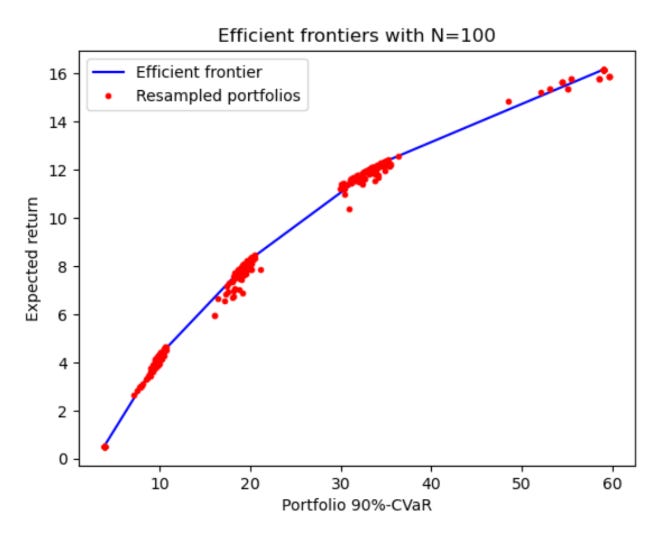
Case Study:
This is a mean-CVaR efficient frontier, and the red dots are the resampled portfolios obtained under parameter uncertainty.
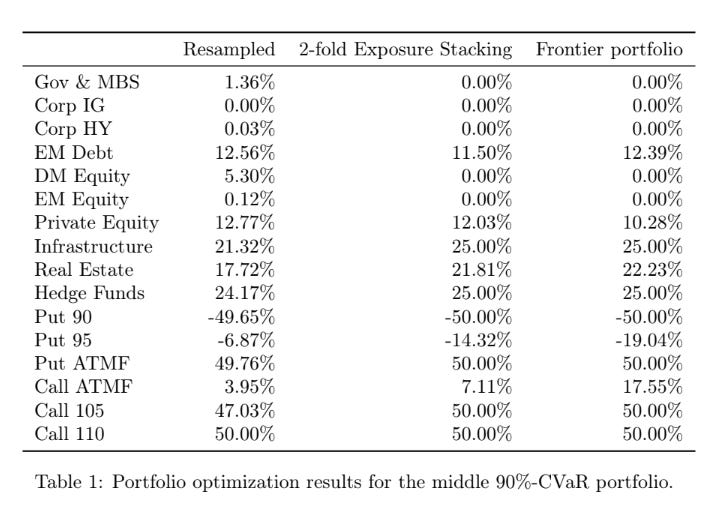
Below is a table comparing the results for the middle 90%-CVaR portfolio constructed using the traditional equal-weight resampled optimization, 2-fold Exposure Stacking, and normal efficient frontier optimization. The author uses a 2-fold Exposure Stacking due to the previous findings from the paper Kristensen and Vorobets (2024), while noting that B = 100 samples is on the lower end of what is recommended in practice.
One of the main problems of traditional resampling is that it generates highly fragmented allocations with a large number of small positions, which is a common sign of averaging noisy portfolio solutions. Exposure Stacking, on the other hand, produces a significantly sparser and more structured portfolio that not only closely matches the efficient frontier allocation but also stays robust against parameter uncertainty.
Exposure Stacking maintains significant derivative exposures—like option convexity—while reducing the effect of noise that drives unstable allocations. This really speaks to the fact that, at the exposure level, aggregation keeps the economic structure of the optimal portfolio, thus, without the fragility and single-model optimization.