Tracking Error is an Estimation Problem, not an Optimization Problem
Why better covariance estimation matters more than clever optimization

Both active and passive investment managers operate relative to their respective benchmarks. For passive investing, the goal is to track or replicate the benchmark, and for active investing, the aim is expose views or tilts, but must ensure they don’t deviate too far from the benchmark. In both cases, a lower tracking error is considered better. The post summarizes the research showing that proper estimation of the covariance matrix (how risk is estimated) is more effective for tracking error management than optimization tricks.
Instead of the Sample Covariance Matrix, the author valued the Shrinkage Estimator combined with the multivariate GARCH model, which leads to significantly better tracking error outcomes. Sample covariance matrices are often noisy and unstable, particularly with a large number of assets and limited data. Whereas shrinkage estimators don’t trust raw historical correlation too much. It denoises the covariance matrix, pulls extreme correlation towards more reasonable values, reduces noise, and improves the out-of-sample performance. Better control over the covariance matrix translates directly into improved tracking error and, ultimately, better portfolio construction.
The paper performed the Optimization using both the unconditional and conditional shrinkage and compared it with the sample covariance matrix. The unconditional shrinkage methods, such as linear shrinkage (Ledoit-Wolf) and Quadratic Inverse Shrinkage (QIS), are better structured when correlations are stable, and the regime doesn’t change constantly. Whereas the conditional shrinkage is applied when volatility and correlation change over time. The multivariate GARCH model and DCC-NL (Dynamic Conditional Correlation-Non Linear Shrinkage) were used to model the time-varying volatility.
In passive portfolio optimization, the objective is to closely replicate the benchmark by minimizing tracking error (TE), which is defined as the volatility of the return difference between the portfolio and the benchmark. With the known benchmark weights, the portfolio manager avoids the illiquid assets and focuses mainly on the smaller liquid subset of assets (the eligible universe).
Sometimes the benchmark weights (and even the constituents) are unknown, but the benchmark return is observable; in this case, we minimize the variance of the difference between the portfolio return and the benchmark return. This leads to the benchmark following or fund-mimicking portfolios.
For active stratergy the most important part is to control the tracking error. The two ways to control the tracking error are
Tracking Error in Objective Function (Soft Control) — The Tracking error is penalized directly in the objective function. The tuning parameter δ ∈ [0,1] controls this balance.
\(\begin{aligned} \max_{w} \;& \delta \cdot \text{active} - (1-\delta)\,(w - w_{BM,t})^\top \Sigma_{r,t} (w - w_{BM,t}) \\ \text{s.t. } \;& w^\top \mathbf{1} = 1 \\ & w_i \ge 0 \end{aligned}\)Tracking Error as Constraint (Hard Control) —This is where the manager maximizes the strategy (active - here the author used GMV as an active strategy) while forcing the TE to stay below the fixed limit. This imposes an upper bound τ on the tracking error variance.
\(\begin{aligned} \max_{w} \;& \text{active} \\ \text{s.t. } \;& w^\top \mathbf{1} = 1 \\ & (w - w_{BM,t})^\top \Sigma_{r,t} (w - w_{BM,t}) \le \tau \\ & w_i \ge 0 \end{aligned}\)
The paper suggested the use of GMV, the global minimum variance, as the active strategy, which seeks lower portfolio risk then benchmark while controlling deviation from the benchmark.
Empirical Analysis
The empirical analysis is conducted using daily stock return data from CRSP spanning 1978–2022 for stocks listed on the NYSE, AMEX, and NASDAQ. Portfolios are rebalanced monthly over an out-of-sample period from February 1983 to December 2022. At each investment date, the investment universe is constructed by selecting up to 1,000 large-capitalization stocks with sufficiently complete return histories, with a subset designated as eligible to ensure liquidity and realistic trading conditions. Covariance matrices are estimated using a rolling window of the most recent 1,260 daily returns (approximately five years), employing alternative estimators including the sample covariance, linear shrinkage, nonlinear shrinkage, and a dynamic correlation GARCH model. Portfolios are then constructed to implement passive minimum-tracking-error strategies and active global minimum-variance strategies with tracking-error penalties or constraints, relative to multiple benchmarks under both known and unknown benchmark-weight settings. Portfolio performance is evaluated using realized and predicted tracking error, volatility, constraint-violation rates, turnover, and leverage, allowing for a comprehensive assessment of tracking-error management and covariance-estimation accuracy.
Passive Minimum TE Portfolios
Exhibit 1 and 2 — Ex Post Tracking Error (Known Benchmark Weights)
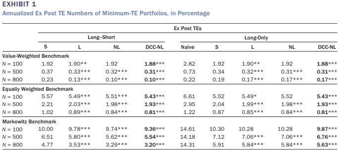
This report shows that the realized (ex post) tracking error of passive minimum-TE portfolios when the benchmark weights are known, the tracking error reduces as the size of the eligible investment universe increases. Which concludes larger the subset of eligible assets closer the replication of the benchmark. The three benchmark has been positioned, the value-weighted benchmark has the lowest tracking error, followed by equal weighted benchmark and the Markowitz benchmark. Allowing the short position is beneficial with a larger universe. These portfolios are constructed using Shrinkage based estimator, and we can see that all the 3 estimators outperformed the sample covariance matrix, DCC-NL achieving the lowest tracking error across all scenarios.
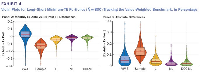
Exhibits 3 and 4 — Ex Ante vs. Ex Post Tracking Error Accuracy
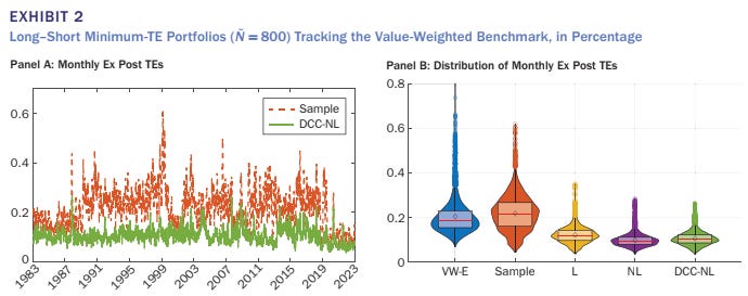
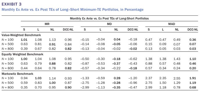
Exhibits 3 and 4 jointly assess how well different covariance estimators forecast tracking error by comparing ex ante (predicted) and ex post (realized) tracking errors for long–short minimum-TE portfolios. Exhibit 3 shows that the sample covariance matrix is the most optimistic and least accurate, exhibiting large biases and high dispersion in forecast errors, whereas nonlinear shrinkage (NL) and DCC-NL consistently produce mean ratios closer to one, smaller biases, and lower absolute deviations. Exhibit 4 provides a graphical confirmation of these results, showing that the distributions of both the signed and absolute differences between ex ante and ex post tracking error are centered closer to zero and significantly tighter for NL and DCC-NL.
Active GMV Portfolios
For active portfolio strategies, tracking error is incorporated as part of the investor’s objective rather than being minimized outright, with all stocks assumed to be investable. Exhibit 6 reports additional portfolio characteristics and shows that shrinkage-based covariance estimators substantially reduce turnover and gross leverage relative to the sample covariance matrix, indicating more stable and implementable active portfolios. Exhibit 7 demonstrates that the superior tracking-error performance of shrinkage estimators—particularly NL and DCC-NL—remains robust even when shorter estimation windows of one or two years are used.
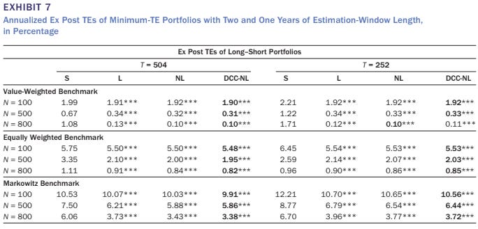
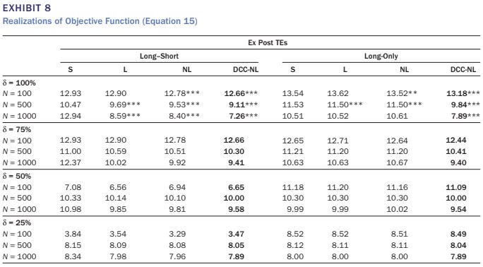
Exhibit 8 evaluates the realized objective function for different trade-offs between active risk and tracking error, showing that DCC-NL consistently delivers the best outcomes, especially as the importance of tracking error increases. Overall, these results confirm that improved covariance estimation enhances not only passive tracking but also the efficiency, stability, and risk control of active portfolio strategies.