Why Simple Feature Selection Beats Deep Learning in Index Tracking
A two-stage framework that matches MIP accuracy while being faster, more stable, and practical

In today’s world, passive investment through index funds and exchange-traded funds (ETFs) is becoming a dominant strategy for many investors. However, replicating these large equity indices like Nifty 50 and S&P500 has always been a practical challenge for the fund managers due to transaction costs, rebalancing overhead, and regulatory constraints. In the paper I’m summarizing here, the author demonstrates how the two-stage feature selection approach outperforms the single-stage MIP approach and the autoencoder model.
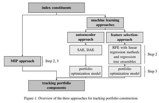
To build a clear view of the feature selection approach, the author set up a 3-stage framework where the core methodology operates in two steps, and the idea is clear: step 2 — Which assets to hold, and step 3 — How much each asset should weigh.
Step 2 focuses on feature selection, that is, deciding which assets to hold from the index constituents so that the framework can track the index with minimal tracking error. In this stage, machine learning based feature selection methods have been used to explicitly select the subset of the assets and also keep control over the portfolio cardinality. Rather than indirectly controlling sparsity through hyperparameters, the number of selected stocks is fixed directly, which is much more practical for real ETF construction.
Step 3 focuses on weight optimization, that is, deciding how much weight each selected asset should receive. After the subset of the asset has been selected from Step 2, a tracking error minimization problem is solved to determine portfolio weights, which includes realistic financial and regulatory constraints for the optimization, making the approach suitable for real-world index tracking.
As in the above framework, the author considers a One-Stage MIP solver as a baseline model. The model solves the Stage 2 and Stage 3 problem together — Selects the subset assets, plus assigns the weights to them. This is computationally very expensive and difficult to scale for the large indices.
In the autoencoder approach, Step 2 is performed using Sparse Autoencoders (SAE) and Denoising Autoencoders (DAE). These models are used to capture the latent space of the market, and stocks are selected based on reconstruction errors. Stocks that are reconstructed well are considered more representative of the index and are selected accordingly.
In contrast, the feature selection approach uses a wrapper-based method called Recursive Feature Elimination (RFE). Least squares regression is used as a baseline, and several supervised learning models are wrapped inside RFE to rank and eliminate stocks. The linear models include least squares, ridge regression (linear with multicollinearity handling), LASSO (sparse linear), elastic net (sparse and correlated), and support vector regression (robust linear). To capture non-linear effects, random forest and XGBoost are used. Each of these models provides feature importance scores, which are used only to rank and remove stocks.
The main objective of the paper is to show that selection and weight optimization are completely isolated. The same classical tracking error optimization model is used after selection, regardless of whether stocks were selected using RFE, autoencoders, or the single-stage MIP approach.
In Step 3, the objective is to minimize tracking error, defined as the squared difference between the tracking portfolio returns and the benchmark index returns. This optimization is subject to a budget constraint, ensuring the portfolio is fully invested, and a long-only constraint, prohibiting short-selling. A cardinality constraint limits the number of stocks in the portfolio, and weight bounds are applied to enforce practicality and diversification. A lower bound of 1e^{−4} avoids tiny, uneconomical holdings, while an upper bound of 5e^{−2} ensures diversification and compliance with UCITS and ICA 1940 regulations.
Key Results
The following paper conducted tests on the S&P500 and CSI300 using daily data from 2006 to 2023 across multiple market regimes.
The Evaluation Criteria include Tracking Difference (TD) — it measures the annualized return gap between the tracking portfolio and the benchmark, Tracking Error (TE) — it is the volatility of the return difference between the tracking portfolio and the benchmark.
The author also suggested the Root Mean Squared Error (RMSE)
Low diversification in the assets or the sector can increase the tracking error in certain market condition which is why the reciprocal Herfindahl-Hirschman-Index (HHI) is also used to measure the portfolio diversification.
Portfolio Turnover — how much the portfolio changes over time, and is directly linked with transaction costs
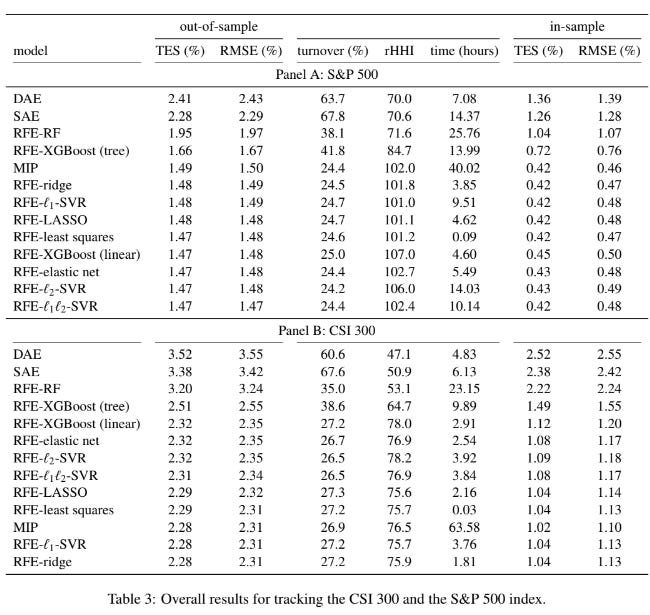
S&P 500 results (Panel A)
Feature selection with linear models and MIP gives almost the same results.
Out-of-sample tracking error is around 1.47%–1.50%, turnover is about 24%–25%, and portfolio diversity sits roughly between 101 and 107. So economically, there is no meaningful difference between MIP and RFE with linear models.
The huge difference is in computing time.
MIP takes ~40 hours.
RFE with least squares takes ~5 minutes.
That’s the main win.
SVR-based RFE is much slower (9–14 hours), and tree-based models like Random Forest and XGBoost (tree) take even longer (14–26 hours) without improving tracking performance. Autoencoders are also slow and clearly worse.
Autoencoders give higher tracking error, very high turnover (~65–70%), and low diversification (~70). Between SAE and DAE, SAE is slightly better, but both are clearly inferior.
CSI 300 results (Panel B)
The CSI 300 shows the same pattern, just with higher tracking errors overall, which makes sense because the market is more volatile and data quality is poorer.
Again, RFE with linear models performs as well as MIP, with out-of-sample tracking errors around 2.28%–2.35%, similar turnover (~27%), and similar diversification (~76–78).
But again, RFE is much faster. Least squares takes ~2 minutes, while MIP takes ~64 hours and does not even reach optimality.
Tree-based models and autoencoders again perform worse, with higher errors and worse portfolio properties.
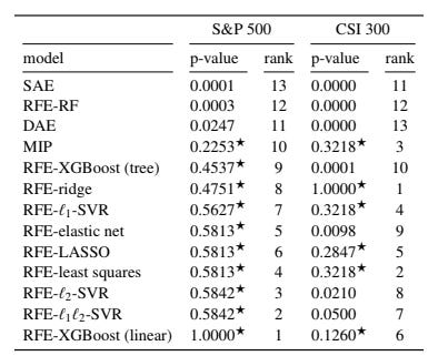
Model Confidence Set (MCS)
To avoid just picking the lowest error model blindly, the authors use a Model Confidence Set (MCS) analysis, which states —
Autoencoders (SAE, DAE) and Random Forest are statistically rejected
Linear RFE models and MIP are statistically indistinguishable
For the S&P 500, RFE-XGBoost (linear) ranks best
For CSI 300, RFE-ridge ranks best
Five linear models
RFE-ridge
RFE-LASSO
RFE-least squares
RFE-l1-SVR,
RFE-XGBoost (linear)
consistently stays inside the confidence set for both datasets.
The final conclusion is that simple feature selection + classical tracking error optimization wins.